How Feature Engineering can help you do well in a Kaggle competition — Part II
In the first part of this series, I introduced the Outbrain Click Prediction machine learning competition. That post described some preliminary and important data science tasks like exploratory data analysis and feature engineering performed for the competition, using a Spark cluster deployed on Google Dataproc.
In this post, I describe the competition evaluation, the design of my cross-validation strategy and my baseline models using statistics and trees ensembles.
Prediction task
In that competition, Kagglers were required to rank recommended ads by decreasing predicted likelihood of being clicked. Sponsored search advertising, contextual advertising, display advertising and real-time bidding auctions have all relied heavily on the ability of learned models to predict ad click-through rates (CTRs) accurately, quickly and reliably.
The evaluation metric was MAP@12 (Mean Average Precision at 12), which measures the ranking quality. In other words, given a set of ads presented during a user visit, this metric assesses whether the clicked ad was ranked by your model on top of other ads. MAP@12 metric is shown below, where |U| is the total number of user visits (display_ids) to a landing page with ads, n is the number of ads on that page, and P(k) is the precision at cutoff k.

This competition made available a very large relational database in CSV format, whose model was shown in the first post. The main tables were clicks_train.csv (~87 million rows) and clicks_test.csv (~32 million rows), representing train set and test set, respectively.
The train set (display_id, ad_id, clicked) contained information about which ads (ad_id) were recommended to a user in a given [landing] page visit (display_id), and which one of the ads was actually clicked by the user. Display_id and ad_id are foreign keys, allowing other tables to join with more context about user visit, landing page and the pages referred by the ads.
The test set (display_id, ad_id) contained the same attributes, except the clicked flag, as expected.
The expected solution was a CSV file with predictions for test set. The first column was the display_id and the second column was a ranked list of ad_ids, split by a space character.
display_id,ad_id
16874594,66758 150083 162754 170392 172888 180797
16874595,8846 30609 143982
16874596,11430 57197 132820 153260 173005 288385 289122 289915
...
Cross-validation
It is always critical to verify whether a machine learning model can generalize beyond the training dataset. Cross-Validation (CV) is an important step to ensure such generalization.
It was necessary to separate from clicks_train.csv a percentage of samples for validation set (about 30%) and the remaining samples as train set. Machine learning models were trained using train set data and their accuracy was evaluated on validation set data, by comparing the predictions with the ground truth labels (clicks).
As we optimize CV model accuracy — by testing different feature engineering approaches, algorithms and hyperparameters tuning — we expect to improve our score on the competition Leaderboard (LB) accordingly (test set).
For most Kaggle competitions, there is a daily submission limit (two in this contest), and CV techniques allow unlimited evaluation of approaches.
For this competition, I used a CV method named holdout, which simply consists of separating a fixed validation set from train set. Another common evaluation strategy is called k-fold, for example.
Time split is also an important aspect when evaluating machine learning models based on human behavior. Many factors might affect users’ interests across time, like recency, search trends and real-world events, among others.
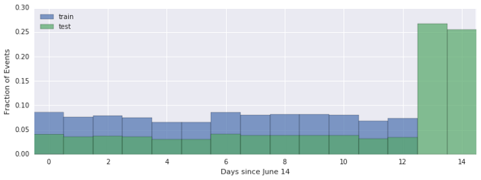
In the figure below, we observe the fraction of events distributed across time (15 days) on train and test sets. About half of the test data (clicks_test.csv) was sampled from the same days as the train set (in-time), with another half being sampled from the two days immediately following representing future predictions (out-of-time).
Based on that observation, my CV strategy was to sample validation set samples according to the same time distribution of test set. Below you can see how that stratified sampling can be easily done using a Spark SQL Dataframe (cluster deployed on Google Dataproc). For the validation set, I sampled 20% of each day, and all events from the last two days (11 and 12).
That careful sampling for validation set did pay off during competition, because my CV score matched the public leaderboard score up to the fourth decimal digit. Thus, I was confident in optimizing my models using the CV score, and only submitting when I could get a significant improvement on it.
Baseline predictions
Up to this point, I had a hard time performing exploratory data analysis, feature engineering and implementing the cross-validation strategy. In my experience, those tasks usually take about 60%-80% of your effort in machine learning projects. And if you get them wrong, they would compromise the maximum accuracy that could be achieved by the models.
Now, let’s switch gears and talk about the predictive algorithms used in this journey. My strategy, focused on personal learning, was to evaluate from simpler to state-of-the-art models in order to assess their upper bound accuracy for this challenge.
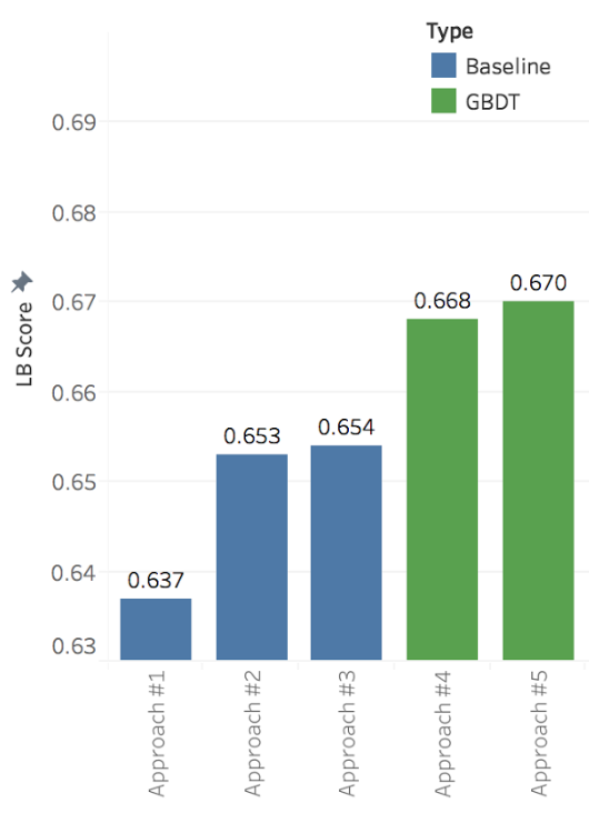
My Approach #1 was already described in the first post of this series, simply using the historical CTR to rank ads, with no machine learning involved. That was a popular baseline approach among the competitors, because it provided an LB score (MAP@12) of 0.637. Just for reference, the official competition baseline was 0.485, obtained by ranking the ads solely by their ids (random-like approach).
The Kaggle community is very generous on shared insights and approaches, even during the competitions. One of the Kagglers shared a data leak he had discovered. That leak, based on the page_views.csv dataset, revealed the actually clicked ads for about 4% user visits (display_ids) of test set. For a machine learning competition, sharing the data leak was kind of a fair-play, and created a new baseline for competitors. My Approach #2 was to use the Approach #1 predictions and only adjust ads ranking for leaked clicked ads, putting them on top of other ads. My LB score then jumped up to 0.65317, and the data leak was used in all my remaining submissions in the competition, as well as the other competitors did.
Most ads had very few views (less than 10) to compute a statistically significant CTR. So, my intuition was that prior knowledge on clicks probability for other categorical values would have some predictive power for unseen events. Thus, I computed average CTR not only for ad ids, but also for other categorical values, that is, P(click | category), and for some two-paired combinations: P(click | category1, category2).
The categorical fields whose average CTR presented higher predictive accuracy on CV score were ad_document_id, ad_source_id, ad_publisher_id, ad_advertiser_id, ad_campain_id, document attributes (category_ids, topics_ids, entities_ids) and their combinations with event_country_id, which modeled regional user preferences.
The CTR confidence was a metric tailored by me during this competition to measure how much a categorical CTR could be used to predict clicks for a specific ad.
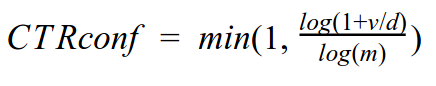
In this equation, d is the number of distinct ads sharing a categorical value, and v was the views count of those ads. A high d value means that a categorical value is too generic to be used for a specific ad (eg. “topic=politics”), leading to a lower CTR confidence.
A high v indicates that ads with that categorical value had many views, increasing CTR statistical significance. For example, the CTR for a specific campaign (categorical value) might be more specific to the ad than using the historical advertiser CTR (higher d), therefore, maybe the campaign had not enough views ( v<10, for example) for statistical significance, leading to a lower confidence on the CTR of a specific campaign when compared to advertiser historical CTR.
L og transformation is also applied to smooth the function for very popular categories/ads. Finally, we normalize the metric to a range between 0.0 and 1.0 by dividing by m, which represent a reference number of average views of distinct ads ( v/d) for maximum confidence (1.0). I used m=100,000 for this competition.
The Approach #3 consisted in a weighted average of all selected CTRs by categories, weighted by their CTR Confidence. That approach improved my LB score to 0.65498.
After manually stressing of those baseline predictors, it was time to start exploring machine learning algorithms to deal with this problem.
Machine learning models
In this section I present the first machine learning models I tried for this challenge: Collaborative Filtering and Trees Ensembles.
Collaborative Filtering — ALS Matrix Factorization
Collaborative Filtering (CF) is probably the most popular technique for recommender systems. CF allow the modeling of users interests by collecting preferences or taste information from many other users (collaborating) to provide personalized recommendations (filtering). Thus, this method was a natural first candidate to be assessed.
Alternating Least Squares (ALS) Matrix Factorization can be applied as a model-based CF for a large matrix of users and items. We used Spark ALS implementation, which features distributed processing across a cluster and supports implicit feedback data (e.g. views, clicks, purchases, likes and shares) as well as explicit feedback data (e.g. movie or books ratings).
The first step was to build a sparse utility matrix of users and documents (content pages referred by ads). The matrix was filled with views count of each document by each user. Log transformation was necessary to smooth views count because some users (or bots) had seen the same web page many times during the 15 days of competition data.
After many attemps tuning Spark’s ALS Matrix Factorization hyperparameters, the best model (presented below) got a Cross-Validation (CV) MAP score of 0.56116, much lower than previous baselines. Thus, this model was not used in my final ensembled solution.
A possible reason for such bad result was the users’ cold-start — the average page views by user was only 2.5, from a collection of more than 2 million pages, making it difficult for a CF approach to infer users preferences and complete such a large and sparse matrix.
Gradient Boosted Decision Trees
Standard CF uses only the utility matrix between users and items (documents). For this competition, there were a vast amount of attributes related to the visit context, the landing page and the ads. Thus, we tried a Learning To Rank approach to take advantage of such rich side information.
The machine learning model employed was Gradient Boosted Decision Trees (GBDT), which is an ensemble of many Decision Trees (weak learners). Similarly to Random Forests (RF), each individual tree is trained with a subsample of the training instances (a.k.a. bagging) and a subsample of the attributes (feature bagging) in order to get individual models with different perspectives of the data. Differently than RF, GBDT assigns more weight to training instances mistakenly classified by previous trees, improving model accuracy and making it a more robust classifier.
I’ve tested two GBDT frameworks, whose implementation was very fast and memory-efficient for large datasets: XGBoost and LightGBM. In our context, they allowed to focus in optimizing the ads ranking for a given user page visit (display_id), instead of trying to predict whether individual ads were clicked or not. XGBoost with ranking objective optimized learning based on MAP metric (the official competition evaluation metric), while LightGBM optimized upon a different ranking metric named NDCG.
The attributes used in XGBoost models, described in more details in the first post, were One-Hot Encoded (OHE) categorical ids, average CTR by categories and their confidences, contextual documents similarity (cosine similarity between landing page profiles — categories, topics, entities — and ad documents profiles), users preference similarity (cosine similarity between user profile and ad documents profile). Such number of attributes, specially OHE categorical ids, lead to very sparse feature vectors, with dimensionality of more than 126,000 positions and only 40 non-zero features.
XGBoost hyperparameters tuning is tricky and this tuning guide was very useful for me. The best XGBoost model ( Approach #4) got a LB score of 0.66821 (hyperparameters shown below) — a large jump over baseline models. That took about three hours to train on a single server with 32 CPUs and 208 GB RAM ( n1-highmem-32 machine type on Google GCE).
For LightGBM models, I used as input data only numerical attributes (CTR and similarities), ignoring OHE categorical fields. Training on such data was pretty fast, under 10 minutes. Surprisingly, I could get with LightGBM (Approach #5) a better model than with XGBoost (LB score of 0.67073). My hypothesis is that the high-dimensional categorical features encoded with OHE made it harder to get a random set of very predictive bagged features for trees building. In fact, some competitors reported single GBDT models with scores above 0.68, using the original categorical ids as provided (no OHE or feature hashing), probably because thousand of trees in the GBDT ensemble were able to ignore the noise and model such ids representation.
I used the LightGBM command line interface for training and predicting the models, and the best hyperparameters I could get for my data are presented below for reference.
objective = lambdarank
boosting_type = gbdt
num_trees = 30
num_leaves = 128
feature_fraction = 0.2
bagging_fraction = 0.2
max_bin = 256
learning_rate = 0.2
label_gain = 1,30
More on part III
Up to this point, my LB score had increased significantly over the baseline, by using some basic statistics and trees ensembles. In the next post of this series, I will describe the most powerful machine models to tackle the Click Prediction problem and the ensemble techniques that took me up to the 19th position on the leaderboard (top 2%).
Originally published at https://medium.com on July 26, 2017.
